Inequality Measurement

Guilherme Jacob, Anthony Damico, and Djalma Pessoa

2022-09-06

Another problem faced by societies is inequality. Economic inequality can have several different meanings: income, education, resources, opportunities, wellbeing, etc. Usually, studies on economic inequality focus on income distribution.

Most inequality data comes from censuses and household surveys. Therefore, in order to produce reliable estimates from this samples, appropriate procedures are necessary.

This chapter presents brief presentations on inequality measures, also providing replication examples if possible. It starts with an initial attempt to measure the inequality between two groups of a population; then, it presents ideas of overall inequality indices, moving from the quintile share ratio to the Lorenz curve and measures derived from it; then, it discusses the concept of entropy and presents inequality measures based on it. Finally, it ends with a discussion regarding which inequality measure should be used.

The Gender Pay Gap (svygpg)

Although the \(GPG\) is not an inequality measure in the usual sense, it can still be an useful instrument to evaluate the discrimination among men and women. Put simply, it expresses the relative difference between the average hourly earnings of men and women, presenting it as a percentage of the average of hourly earnings of men.

In mathematical terms, this index can be described as,

\[ GPG = \frac{ \bar{y}_{male} - \bar{y}_{female} }{ \bar{y}_{male} } \],

which is precisely the estimator used in the package. As we can see from the formula, if there is no difference among classes, \(GPG = 0\). Else, if \(GPG > 0\), it means that the average hourly income received by women are \(GPG\) percent smaller than men’s. For negative \(GPG\), it means that women’s hourly earnings are \(GPG\) percent larger than men’s. In other words, the larger the \(GPG\), larger is the shortfall of women’s hourly earnings.

We can also develop a more straightforward idea: for every $1 raise in men’s hourly earnings, women’s hourly earnings are expected to increase $\((1-GPG)\). For instance, assuming \(GPG = 0.8\), for every $1.00 increase in men’s average hourly earnings, women’s hourly earnings would increase only $0.20.

The details of the linearization of the GPG are discussed by Deville (1999) and Osier (2009).

---

A replication example

The R vardpoor package (Breidaks, Liberts, and Ivanova 2016), created by researchers at the Central Statistical Bureau of Latvia, includes a gpg coefficient calculation using the ultimate cluster method. The example below reproduces those statistics.

Load and prepare the same data set:

# load the convey package
library(convey)

# load the survey library
library(survey)
#> Loading required package: grid
#> Loading required package: Matrix
#> Loading required package: survival
#> 
#> Attaching package: 'survey'
#> The following object is masked from 'package:graphics':
#> 
#>     dotchart

# load the vardpoor library
library(vardpoor)

# load the laeken library
library(laeken)

# load the synthetic EU statistics on income & living conditions
data(eusilc)

# make all column names lowercase
names( eusilc ) <- tolower( names( eusilc ) )

# coerce the gender variable to numeric 1 or 2
eusilc$one_two <- as.numeric( eusilc$rb090 == "female" ) + 1

# add a column with the row number
dati <- data.table::data.table(IDd = 1 : nrow(eusilc), eusilc)

# calculate the gpg coefficient
# using the R vardpoor library
varpoord_gpg_calculation <-
    varpoord(
    
        # analysis variable
        Y = "eqincome", 
        
        # weights variable
        w_final = "rb050",
        
        # row number variable
        ID_level1 = "IDd",
        
        # row number variable
        ID_level2 = "IDd",
        
        # strata variable
        H = "db040", 
        
        N_h = NULL ,
        
        # clustering variable
        PSU = "rb030", 
        
        # data.table
        dataset = dati, 
        
        # gpg coefficient function
        type = "lingpg" ,
        
        # gender variable
        gender = "one_two",
      
      # poverty threshold range
      order_quant = 50L ,
      
      # get linearized variable
      outp_lin = TRUE
    )



# construct a survey.design
# using our recommended setup
des_eusilc <- 
    svydesign( 
        ids = ~ rb030 , 
        strata = ~ db040 ,  
        weights = ~ rb050 , 
        data = eusilc
    )

# immediately run the convey_prep function on it
des_eusilc <- convey_prep( des_eusilc )

# coefficients do match
varpoord_gpg_calculation$all_result$value
#> [1] 7.645389
coef( svygpg( ~ eqincome , des_eusilc , sex = ~ rb090 ) ) * 100
#> eqincome 
#> 7.645389

# linearized variables do match
# vardpoor
lin_gpg_varpoord<- varpoord_gpg_calculation$lin_out$lin_gpg
# convey 
lin_gpg_convey <- attr(svygpg( ~ eqincome , des_eusilc, sex = ~ rb090 ),"lin")

# check equality
all.equal(lin_gpg_varpoord,100*lin_gpg_convey[,1] )
#> [1] TRUE

# variances do not match exactly
attr( svygpg( ~ eqincome , des_eusilc , sex = ~ rb090 ) , 'var' ) * 10000
#>           eqincome
#> eqincome 0.6493911
varpoord_gpg_calculation$all_result$var
#> [1] 0.6482346

# standard errors do not match exactly
varpoord_gpg_calculation$all_result$se
#> [1] 0.8051301
SE( svygpg( ~ eqincome , des_eusilc , sex = ~ rb090 ) ) * 100
#>           eqincome
#> eqincome 0.8058481

The variance estimate is computed by using the approximation defined in @ref(eq:var), where the linearized variable \(z\) is defined by @ref(eq:lin). The functions convey::svygpg and vardpoor::lingpg produce the same linearized variable \(z\).

However, the measures of uncertainty do not line up, because library(vardpoor) defaults to an ultimate cluster method that can be replicated with an alternative setup of the survey.design object.

# within each strata, sum up the weights
cluster_sums <- aggregate( eusilc$rb050 , list( eusilc$db040 ) , sum )

# name the within-strata sums of weights the `cluster_sum`
names( cluster_sums ) <- c( "db040" , "cluster_sum" )

# merge this column back onto the data.frame
eusilc <- merge( eusilc , cluster_sums )

# construct a survey.design
# with the fpc using the cluster sum
des_eusilc_ultimate_cluster <- 
    svydesign( 
        ids = ~ rb030 , 
        strata = ~ db040 ,  
        weights = ~ rb050 , 
        data = eusilc , 
        fpc = ~ cluster_sum 
    )

# again, immediately run the convey_prep function on the `survey.design`
des_eusilc_ultimate_cluster <- convey_prep( des_eusilc_ultimate_cluster )

# matches
attr( svygpg( ~ eqincome , des_eusilc_ultimate_cluster , sex = ~ rb090 ) , 'var' ) * 10000
#>           eqincome
#> eqincome 0.6482346
varpoord_gpg_calculation$all_result$var
#> [1] 0.6482346

# matches
varpoord_gpg_calculation$all_result$se
#> [1] 0.8051301
SE( svygpg( ~ eqincome , des_eusilc_ultimate_cluster , sex = ~ rb090 ) ) * 100
#>           eqincome
#> eqincome 0.8051301

For additional usage examples of svygpg, type ?convey::svygpg in the R console.

Quintile Share Ratio (svyqsr)

Unlike the previous measure, the quintile share ratio is an inequality measure in itself, depending only of the income distribution to evaluate the degree of inequality. By definition, it can be described as the ratio between the income share held by the richest 20% and the poorest 20% of the population.

In plain terms, it expresses how many times the wealthier part of the population are richer than the poorest part. For instance, a \(QSR = 4\) implies that the upper class owns 4 times as much of the total income as the poor.

The quintile share ratio can be modified to a more general function of fractile share ratios. For instance, Cobham, Schlogl, and Sumner (2015) presents interesting arguments for using the Palma index, defined as the ratio between the share of the 10% richest over the share held by the poorest 40%.

The details of the linearization of the QSR are discussed by Deville (1999) and Osier (2009).

---

A replication example

The R vardpoor package (Breidaks, Liberts, and Ivanova 2016), created by researchers at the Central Statistical Bureau of Latvia, includes a qsr coefficient calculation using the ultimate cluster method. The example below reproduces those statistics.

Load and prepare the same data set:

# load the convey package
library(convey)

# load the survey library
library(survey)

# load the vardpoor library
library(vardpoor)

# load the laeken library
library(laeken)

# load the synthetic EU statistics on income & living conditions
data(eusilc)

# make all column names lowercase
names( eusilc ) <- tolower( names( eusilc ) )

# add a column with the row number
dati <- data.table::data.table(IDd = 1 : nrow(eusilc), eusilc)

# calculate the qsr coefficient
# using the R vardpoor library
varpoord_qsr_calculation <-
    varpoord(
    
        # analysis variable
        Y = "eqincome", 
        
        # weights variable
        w_final = "rb050",
        
        # row number variable
        ID_level1 = "IDd",
        
        # row number variable
        ID_level2 = "IDd",
        
        # strata variable
        H = "db040", 
        
        N_h = NULL ,
        
        # clustering variable
        PSU = "rb030", 
        
        # data.table
        dataset = dati, 
        
        # qsr coefficient function
        type = "linqsr",
      
      # poverty threshold range
      order_quant = 50L ,
      
      # get linearized variable
      outp_lin = TRUE
        
    )



# construct a survey.design
# using our recommended setup
des_eusilc <- 
    svydesign( 
        ids = ~ rb030 , 
        strata = ~ db040 ,  
        weights = ~ rb050 , 
        data = eusilc
    )

# immediately run the convey_prep function on it
des_eusilc <- convey_prep( des_eusilc )

# coefficients do match
varpoord_qsr_calculation$all_result$value
#> [1] 3.970004
coef( svyqsr( ~ eqincome , des_eusilc ) )
#> eqincome 
#> 3.970004

# linearized variables do match
# vardpoor
lin_qsr_varpoord<- varpoord_qsr_calculation$lin_out$lin_qsr
# convey 
lin_qsr_convey <- 
  as.numeric(
    attr(
        svyqsr( 
            ~ eqincome , 
            des_eusilc , 
            linearized = TRUE  
          ) , 
        "linearized"
    )
  )

# check equality
all.equal(lin_qsr_varpoord, lin_qsr_convey )
#> [1] TRUE

# variances do not match exactly
attr( svyqsr( ~ eqincome , des_eusilc ) , 'var' )
#>             eqincome
#> eqincome 0.001810537
varpoord_qsr_calculation$all_result$var
#> [1] 0.001807323

# standard errors do not match exactly
varpoord_qsr_calculation$all_result$se
#> [1] 0.04251263
SE( svyqsr( ~ eqincome , des_eusilc ) )
#>            eqincome
#> eqincome 0.04255041

The variance estimate is computed by using the approximation defined in @ref(eq:var), where the linearized variable \(z\) is defined by @ref(eq:lin). The functions convey::svygpg and vardpoor::lingpg produce the same linearized variable \(z\).

However, the measures of uncertainty do not line up, because library(vardpoor) defaults to an ultimate cluster method that can be replicated with an alternative setup of the survey.design object.

# within each strata, sum up the weights
cluster_sums <- aggregate( eusilc$rb050 , list( eusilc$db040 ) , sum )

# name the within-strata sums of weights the `cluster_sum`
names( cluster_sums ) <- c( "db040" , "cluster_sum" )

# merge this column back onto the data.frame
eusilc <- merge( eusilc , cluster_sums )

# construct a survey.design
# with the fpc using the cluster sum
des_eusilc_ultimate_cluster <- 
    svydesign( 
        ids = ~ rb030 , 
        strata = ~ db040 ,  
        weights = ~ rb050 , 
        data = eusilc , 
        fpc = ~ cluster_sum 
    )

# again, immediately run the convey_prep function on the `survey.design`
des_eusilc_ultimate_cluster <- convey_prep( des_eusilc_ultimate_cluster )

# matches
attr( svyqsr( ~ eqincome , des_eusilc_ultimate_cluster ) , 'var' )
#>             eqincome
#> eqincome 0.001807323
varpoord_qsr_calculation$all_result$var
#> [1] 0.001807323

# matches
varpoord_qsr_calculation$all_result$se
#> [1] 0.04251263
SE( svyqsr( ~ eqincome , des_eusilc_ultimate_cluster ) )
#>            eqincome
#> eqincome 0.04251263

For additional usage examples of svyqsr, type ?convey::svyqsr in the R console.

Lorenz Curve (svylorenz)

Though not an inequality measure in itself, the Lorenz curve is a classic instrument of distribution analysis. Basically, it is a function that associates a cumulative share of the population to the share of the total income it owns. In mathematical terms,

\[ L(p) = \frac{\int_{-\infty}^{Q_p}yf(y)dy}{\int_{-\infty}^{+\infty}yf(y)dy} \]

where \(Q_p\) is the quantile \(p\) of the population.

The two extreme distributive cases are

• Perfect equality:
  • Every individual has the same income;
  • Every share of the population has the same share of the income;
  • Therefore, the reference curve is \[L(p) = p \text{ } \forall p \in [0,1] \text{.}\]
• Perfect inequality:
  • One individual concentrates all of society’s income, while the other individuals have zero income;
  • Therefore, the reference curve is

\[ L(p)= \begin{cases} 0, &\forall p < 1 \\ 1, &\text{if } p = 1 \text{.} \end{cases} \]

In order to evaluate the degree of inequality in a society, the analyst looks at the distance between the real curve and those two reference curves.

The estimator of this function was derived by Kovacevic and Binder (1997):

\[ L(p) = \frac{ \sum_{i \in S} w_i \cdot y_i \cdot \delta \{ y_i \le \widehat{Q}_p \}}{\widehat{Y}}, \text{ } 0 \le p \le 1. \]

Yet, this formula is used to calculate specific points of the curve and their respective SEs. The formula to plot an approximation of the continuous empirical curve comes from Lerman and Yitzhaki (1989).

---

A replication example

In October 2016, (Jann 2016) released a pre-publication working paper to estimate lorenz and concentration curves using stata. The example below reproduces the statistics presented in his section 4.1.

# load the convey package
library(convey)

# load the survey library
library(survey)

# load the stata-style webuse library
library(webuse)

# load the NLSW 1988 data
webuse("nlsw88")

# coerce that `tbl_df` to a standard R `data.frame`
nlsw88 <- data.frame( nlsw88 )

# initiate a linearized survey design object
des_nlsw88 <- svydesign( ids = ~1 , data = nlsw88 )
#> Warning in svydesign.default(ids = ~1, data = nlsw88): No weights or
#> probabilities supplied, assuming equal probability

# immediately run the `convey_prep` function on the survey design
des_nlsw88 <- convey_prep(des_nlsw88)

# estimates lorenz curve
result.lin <- svylorenz( ~wage, des_nlsw88, quantiles = seq( 0, 1, .05 ), na.rm = TRUE )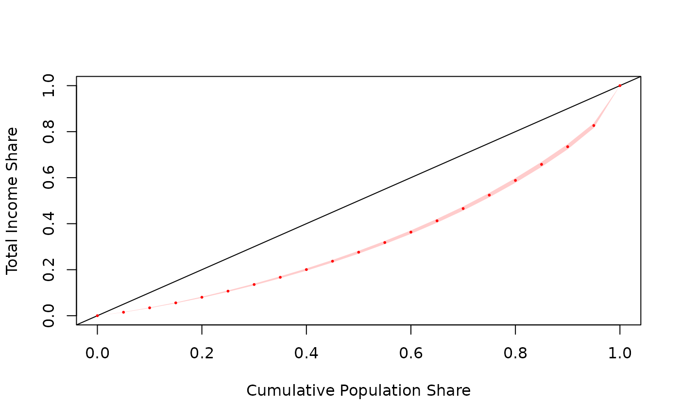

# note: most survey commands in R use Inf degrees of freedom by default
# stata generally uses the degrees of freedom of the survey design.
# therefore, while this extended syntax serves to prove a precise replication of stata
# it is generally not necessary.
section_four_one <-
    data.frame( 
        estimate = coef( result.lin ) , 
        standard_error = SE( result.lin ) , 
        ci_lower_bound = 
            coef( result.lin ) + 
            SE( result.lin ) * 
            qt( 0.025 , degf( subset( des_nlsw88 , !is.na( wage ) ) ) ) ,
        ci_upper_bound = 
            coef( result.lin ) + 
            SE( result.lin ) * 
            qt( 0.975 , degf( subset( des_nlsw88 , !is.na( wage ) ) ) )
    )
    

	estimate	standard_error	ci_lower_bound	ci_upper_bound
L(0)	0.0000000	0.0000000	0.0000000	0.0000000
L(0.05)	0.0151060	0.0004159	0.0142904	0.0159216
L(0.1)	0.0342651	0.0007021	0.0328882	0.0356420
L(0.15)	0.0558635	0.0010096	0.0538836	0.0578434
L(0.2)	0.0801846	0.0014032	0.0774329	0.0829363
L(0.25)	0.1067687	0.0017315	0.1033732	0.1101642
L(0.3)	0.1356307	0.0021301	0.1314535	0.1398078
L(0.35)	0.1670287	0.0025182	0.1620903	0.1719670
L(0.4)	0.2005501	0.0029161	0.1948315	0.2062687
L(0.45)	0.2369209	0.0033267	0.2303971	0.2434447
L(0.5)	0.2759734	0.0037423	0.2686347	0.2833121
L(0.55)	0.3180215	0.0041626	0.3098585	0.3261844
L(0.6)	0.3633071	0.0045833	0.3543192	0.3722950
L(0.65)	0.4125183	0.0050056	0.4027021	0.4223345
L(0.7)	0.4657641	0.0054137	0.4551478	0.4763804
L(0.75)	0.5241784	0.0058003	0.5128039	0.5355529
L(0.8)	0.5880894	0.0062464	0.5758401	0.6003388
L(0.85)	0.6577051	0.0066148	0.6447333	0.6706769
L(0.9)	0.7346412	0.0068289	0.7212497	0.7480328
L(0.95)	0.8265786	0.0062686	0.8142857	0.8388715
L(1)	1.0000000	0.0000000	1.0000000	1.0000000

For additional usage examples of svylorenz, type ?convey::svylorenz in the R console.

Gini index (svygini)

The Gini index is an attempt to express the inequality presented in the Lorenz curve as a single number. In essence, it is twice the area between the equality curve and the real Lorenz curve. Put simply:

\[ \begin{aligned} G &= 2 \bigg( \int_{0}^{1} pdp - \int_{0}^{1} L(p)dp \bigg) \\ \therefore G &= 1 - 2 \int_{0}^{1} L(p)dp \end{aligned} \]

where \(G=0\) in case of perfect equality and \(G = 1\) in the case of perfect inequality.

The estimator proposed by Osier (2009) is defined as:

\[ \widehat{G} = \frac{ 2 \sum_{i \in S} w_i r_i y_i - \sum_{i \in S} w_i y_i }{ \hat{Y} } \]

The linearized formula of \(\widehat{G}\) is used to calculate the SE.

---

A replication example

The R vardpoor package (Breidaks, Liberts, and Ivanova 2016), created by researchers at the Central Statistical Bureau of Latvia, includes a gini coefficient calculation using the ultimate cluster method. The example below reproduces those statistics.

Load and prepare the same data set:

# load the convey package
library(convey)

# load the survey library
library(survey)

# load the vardpoor library
library(vardpoor)

# load the laeken library
library(laeken)

# load the synthetic EU statistics on income & living conditions
data(eusilc)

# make all column names lowercase
names( eusilc ) <- tolower( names( eusilc ) )

# add a column with the row number
dati <- data.table::data.table(IDd = 1 : nrow(eusilc), eusilc)

# calculate the gini coefficient
# using the R vardpoor library
varpoord_gini_calculation <-
    varpoord(
    
        # analysis variable
        Y = "eqincome", 
        
        # weights variable
        w_final = "rb050",
        
        # row number variable
        ID_level1 = "IDd",
        
        # row number variable
        ID_level2 = "IDd",
        
        # strata variable
        H = "db040", 
        
        N_h = NULL ,
        
        # clustering variable
        PSU = "rb030", 
        
        # data.table
        dataset = dati, 
        
        # gini coefficient function
        type = "lingini",
      
      # poverty threshold range
      order_quant = 50L ,
      
      # get linearized variable
      outp_lin = TRUE
        
    )



# construct a survey.design
# using our recommended setup
des_eusilc <- 
    svydesign( 
        ids = ~ rb030 , 
        strata = ~ db040 ,  
        weights = ~ rb050 , 
        data = eusilc
    )

# immediately run the convey_prep function on it
des_eusilc <- convey_prep( des_eusilc )

# coefficients do match
varpoord_gini_calculation$all_result$value
#> [1] 26.49652
coef( svygini( ~ eqincome , des_eusilc ) ) * 100
#> eqincome 
#> 26.49652

# linearized variables do match
# varpoord
lin_gini_varpoord<- varpoord_gini_calculation$lin_out$lin_gini
# convey 
lin_gini_convey <- attr( svygini( ~ eqincome , des_eusilc , linearized = TRUE ) , "linearized" )

# check equality
all.equal( lin_gini_varpoord , ( 100 * as.numeric( lin_gini_convey ) ) )
#> [1] TRUE

# variances do not match exactly
attr( svygini( ~ eqincome , des_eusilc ) , 'var' ) * 10000
#>            eqincome
#> eqincome 0.03790739
varpoord_gini_calculation$all_result$var
#> [1] 0.03783931

# standard errors do not match exactly
varpoord_gini_calculation$all_result$se
#> [1] 0.1945233
SE( svygini( ~ eqincome , des_eusilc ) ) * 100
#>           eqincome
#> eqincome 0.1946982

The variance estimate is computed by using the approximation defined in @ref(eq:var), where the linearized variable \(z\) is defined by @ref(eq:lin). The functions convey::svygini and vardpoor::lingini produce the same linearized variable \(z\).

However, the measures of uncertainty do not line up, because library(vardpoor) defaults to an ultimate cluster method that can be replicated with an alternative setup of the survey.design object.

# within each strata, sum up the weights
cluster_sums <- aggregate( eusilc$rb050 , list( eusilc$db040 ) , sum )

# name the within-strata sums of weights the `cluster_sum`
names( cluster_sums ) <- c( "db040" , "cluster_sum" )

# merge this column back onto the data.frame
eusilc <- merge( eusilc , cluster_sums )

# construct a survey.design
# with the fpc using the cluster sum
des_eusilc_ultimate_cluster <- 
    svydesign( 
        ids = ~ rb030 , 
        strata = ~ db040 ,  
        weights = ~ rb050 , 
        data = eusilc , 
        fpc = ~ cluster_sum 
    )

# again, immediately run the convey_prep function on the `survey.design`
des_eusilc_ultimate_cluster <- convey_prep( des_eusilc_ultimate_cluster )

# matches
attr( svygini( ~ eqincome , des_eusilc_ultimate_cluster ) , 'var' ) * 10000
#>            eqincome
#> eqincome 0.03783931
varpoord_gini_calculation$all_result$var
#> [1] 0.03783931

# matches
varpoord_gini_calculation$all_result$se
#> [1] 0.1945233
SE( svygini( ~ eqincome , des_eusilc_ultimate_cluster ) ) * 100
#>           eqincome
#> eqincome 0.1945233

Zenga index (svyzenga)

Proposed by Zenga (2007), the Zenga index is another inequality measure related to the Lorenz curve with interesting properties. For continuous populations, it is defined as:

\[ Z = 1 - \int_{0}^{1} \frac{L(p)}{p} \cdot \frac{ 1 - p }{ 1 - L(p) } dp \]

In practice, convey uses the Barabesi, Diana, and Perri (2016) estimator, based on the finite population Zenga index, and a variance estimator derived using Deville’s (1999) influence function method.

Alternatively, Langel and Tillé (2012) uses an estimator based on smoothed quantiles and a variance estimator based on Demnati and Rao (2004) linearization method. However, Barabesi, Diana, and Perri (2016) finds that both estimators behave very similarly.

The intuition behind the Zenga index is based on argument similar to the Quintile Share Ratio or Palma index. While the QSR and Palma indices are based on ratios of bottom and upper shares, the Zenga scores (but not the measure itself!) is the ratio of bottom and upper means. The Zenga index is the average of those scores.

For a given p, when the mean income of the poorest is not much smaller than the mean income of the richest, the ratio is close to one, resulting in Z(p) close to zero. However, when the bottom mean is much smaller than the upper mean, the ratio goes to 0, resulting in a Z(p) close to one.

Take the poorest 20%: the mean income of the poorest 20%, this is the lower mean. The “complement” is the mean income of the richest 80%: this is the upper mean. If the lower mean is $100 and the upper mean is $1,000, then the respective point on the Zenga curve would associate the fraction 20% to 1 - ( $100 / $1,000 ) = 0.9. In other words, Z(20%) = 90%.

In this case, we took a fixed p = 20%; however, the full Zenga curve would be computed varying p from 0% to 100%. Then, the Zenga index is the integral of this curve in the interval (0,1).

Unlike the relationship between the Gini coefficient and the Lorenz curve, this allows for a more straightforward graphical interpretation (see Figure 1 from Langel and Tillé (2012)) of the Zenga index. In fact, the Zenga index is the mean of the Y axis of the Zenga coordinates.

According to Langel and Tillé (2012), “the Zenga index is significantly less affected by extreme observations than the Gini index. This is a very important advantage of the Zenga index because inference from income data is often confronted with extreme values.”

---

A replication example

While it is not possible to reproduce the exact results because their simulation includes random sampling, we can replicate a Monte Carlo experiment similar to the one presented by Barabesi, Diana, and Perri (2016) in Table 2.

Load and prepare the data set:

# load the convey package
library(convey)

# load the survey library
library(survey)

# create a temporary file on the local disk
tf <- tempfile()

# store the location of the zip file
data_zip <- "https://www.bancaditalia.it/statistiche/tematiche/indagini-famiglie-imprese/bilanci-famiglie/distribuzione-microdati/documenti/ind12_ascii.zip"

# download to the temporary file
download.file( data_zip , tf , mode = 'wb' )

# unzip the contents of the archive to a temporary directory
td <- file.path( tempdir() , "shiw2012" )
data_files <- unzip( tf , exdir = td )

# load the household, consumption and income from SHIW (2012) survey data
hhr.df <- read.csv( grep( "carcom12" , data_files , value = TRUE ) )
cns.df <- read.csv( grep( "risfam12" , data_files , value = TRUE ) )
inc.df <- read.csv( grep( "rper12" , data_files , value = TRUE ) )

# fixes names
colnames( cns.df )[1] <- tolower( colnames( cns.df ) )[1]

# household count should be 8151
stopifnot( sum( !duplicated( hhr.df$nquest ) ) == 8151 )

# person count should be 20022
stopifnot( sum( !duplicated( paste0( hhr.df$nquest , "-" , hhr.df$nord ) ) ) == 20022 )

# income recipients: should be 12986
stopifnot( sum( hhr.df$PERC ) == 12986 )

# combine household roster and income datasets
pop.df <- 
    merge( 
        hhr.df , 
        inc.df , 
        by = c( "nquest" ,"nord" ) , 
        all.x = TRUE , 
        sort = FALSE 
    )

# compute household-level income
hinc.df <- 
    pop.df[ 
        pop.df$PERC == 1 , 
        c( "nquest" , "nord" , "PERC" , "Y" , "YL" , "YM" , "YT" , "YC" ) , 
        drop = FALSE 
    ]
    
hinc.df <- 
    aggregate( 
        rowSums( 
            hinc.df[ , c( "YL"  , "YM" , "YT"  ) , drop = FALSE ] 
        ) , 
        list( "nquest" = hinc.df$nquest ) , 
        sum , 
        na.rm = TRUE 
    )
    
pop.df <- 
    merge( 
        pop.df , 
        hinc.df , 
        by = "nquest" , 
        all.x = TRUE , 
        sort = FALSE 
    )

# combine with consumption data
pop.df <- 
    merge( 
        pop.df , 
        cns.df , 
        by = "nquest" , 
        all.x = TRUE , 
        sort = FALSE 
    )

# treat household-level sample as the finite population
pop.df <- 
    pop.df[ !duplicated( pop.df$nquest ) , , drop = FALSE ]

For the Monte Carlo experiment, we take 5000 samples of (expected) size 1000 using Poisson sampling¹ and estimate the Zenga index using each sample:

# set up monte carlo attributes
MC.reps <- 5000L
n.size = 1000L
N.size = nrow( pop.df )

# calculate first order probabilities
pop.df$pik <-
    n.size * ( abs( pop.df$C ) / sum( abs( pop.df$C ) ) )

# calculate second order probabilities
pikl <- pop.df$pik %*% t( pop.df$pik )
diag( pikl ) <- pop.df$pik 

# set random number seed
set.seed( 1997 )

# create list of survey design objects
# using poisson sampling
survey.list <- 
    lapply( 
        seq_len( MC.reps ) , 
        function( this.rep ){
            smp.ind <- which( runif( N.size ) <= pop.df$pik )
            smp.df <- pop.df[ smp.ind , , drop = FALSE ]
            svydesign( 
                ids = ~nquest , 
                data = smp.df , 
                fpc = ~pik , 
                nest = FALSE , 
                pps = ppsmat( pikl[ smp.ind , smp.ind ] ) , 
                variance = "HT" 
            )
        }
    )

# estimate zenga index for each sample
estimate.list <- 
    lapply(
        survey.list , 
        function( this.sample ){
            svyzenga( 
                ~x , 
                subset( this.sample , x > 0 ) , 
                na.rm = TRUE 
            )
        }
    )
    

Then, we evaluate the Percentage Relative Bias (PRB) of the Zenga index estimator. Under this scenario, the PRB of the Zenga index estimator is 0.3397%, a result similar to the 0.321 shown in Table 2.

# compute the (finite population) Zenga index parameter
theta.pop <- convey:::CalcZenga( pop.df$x , ifelse( pop.df$x > 0 , 1 , 0 ) )

# estimate the expected value of the Zenga index estimator
# using the average of the estimates
theta.exp <- mean( sapply( estimate.list , coef ) )

# estimate the percentage relative bias
100 * ( theta.exp/theta.pop - 1 )
#> [1] 0.3396837

Then, we evaluate the PRB of the variance estimator of the Zenga index estimator. Under this scenario, the PRB of the Zenga index variance estimator is -0.4954%, another result similar to the -0.600 shown in Table 2.

# estimate the variance of the Zenga index estimator
# using the variance of the estimates
( vartheta.popest <- var( sapply( estimate.list , coef ) ) )
#> [1] 9.47244e-05

# estimate the expected value of the Zenga index variance estimator
# using the expected of the variance estimates
( vartheta.exp <- mean( sapply( estimate.list , vcov ) ) )
#> [1] 9.425515e-05

# estimate the percentage relative bias
100 * ( vartheta.exp/vartheta.popest - 1 )
#> [1] -0.4953863

Next, we evaluate the Percentage Coverage Rate (PCR). In theory, under repeated sampling, the estimated 95% CIs should cover the population parameter 95% of the time. We can evaluate that using:

# estimate confidence intervals of the Zenga index
# for each of the samples
est.cis <- t( sapply( estimate.list, function( this.stat ) c( confint( this.stat ) ) ) ) 

# evaluate
prop.table( table( ( theta.pop > est.cis[,1] ) & ( theta.pop < est.cis[,2] ) ) )
#> 
#>  FALSE   TRUE 
#> 0.0548 0.9452

Our estimated 95% CIs cover the parameter 94.52% of the time, which is very close to the nominal rate and also similar to the 94.5 PCR shown in Table 2.

Entropy-based Measures

Entropy is a concept derived from information theory, meaning the expected amount of information given the occurrence of an event. Following (Shannon 1948), given an event \(y\) with probability density function \(f(\cdot)\), the information content given the occurrence of \(y\) can be defined as \(g(f(y)) \colon= - \log f(y)\). Therefore, the expected information or, put simply, the entropy is

\[ H(f) \colon = -E \big[ \log f(y) \big] = - \int_{-\infty}^{\infty} f(y) \log f(y) dy \]

Assuming a discrete distribution, with \(p_k\) as the probability of occurring event \(k \in K\), the entropy formula takes the form:

\[ H = - \sum_{k \in K} p_k \log p_k \text{.} \]

The main idea behind it is that the expected amount of information of an event is inversely proportional to the probability of its occurrence. In other words, the information derived from the observation of a rare event is higher than of the information of more probable events.

Using ideas presented in Frank A. Cowell, Flachaire, and Bandyopadhyay (2009), substituting the density function by the income share of an individual \(s(q) = {F}^{-1}(q) / \int_{0}^{1} F^{-1}(t)dt = y/\mu\), the entropy function becomes the Theil² inequality index

\[ I_{Theil} = \int_{0}^{\infty} \frac{y}{\mu} \log \bigg( \frac{y}{\mu} \bigg) dF(y) = -H(s) \]

Therefore, the entropy-based inequality measure increases as a person’s income \(y\) deviates from the mean \(\mu\). This is the basic idea behind entropy-based inequality measures.

Generalized Entropy and Decomposition (svygei, svygeidec)

Using a generalization of the information function, now defined as \(g(f) = \frac{1}{\alpha-1} [ 1 - f^{\alpha - 1} ]\), the \(\alpha\)-class entropy is \[ H^{(\alpha)} (f) = \frac{1}{\alpha - 1} \bigg[ 1 - \int_{-\infty}^{\infty} f(y)^{ \alpha - 1} f(y) dy \bigg] \text{.} \]

This relates to a class of inequality measures, the Generalized entropy indices, defined as:

\[ GE^{(\alpha)} = \frac{1}{\alpha^2 - \alpha} \int_{0}^\infty \bigg[ \bigg( \frac{y}{\mu} \bigg)^\alpha - 1 \bigg]dF(x) = - \frac{-H_\alpha(s) }{ \alpha } \text{.} \]

The parameter \(\alpha\) also has an economic interpretation: as \(\alpha\) increases, the influence of top incomes upon the index increases. In some cases, this measure takes special forms, such as mean log deviation and the aforementioned Theil index.

Biewen and Jenkins (2003) use the following finite-population as the basis for a plugin estimator:

\[ GE^{(\alpha)} = \begin{cases} ( \alpha^2 - \alpha)^{-1} \big[ U_0^{\alpha - 1} U_1^{-\alpha} U_\alpha -1 \big], & \text{if } \alpha \in \mathbb{R} \setminus \{0,1\} \\ - T_0 U_0^{-1} + \log ( U_1 / U_0 ), &\text{if } \alpha \rightarrow 0 \\ T_1 U_1^{-1} - \log ( U_1 / U_0 ), & \text{if } \alpha \rightarrow 1 \end{cases} \]

where \(U_\gamma = \sum_{i \in U} y_i^\gamma\) and \(T_\gamma = \sum_{i \in U} y_i^\gamma \log y_i\). Since those are all functions of totals, the linearization of the indices are easily achieved using the theorems described in Deville (1999).

This class also has several desirable properties, such as additive decomposition. The additive decomposition allows to compare the effects of inequality within and between population groups on the population inequality. Put simply, taking \(G\) groups, an additive decomposable index allows for:

\[ \begin{aligned} I ( \mathbf{y} ) &= I_{Within} + I_{Between} \\ \end{aligned} \]

where \(I_{Within} = \sum_{g \in G} W_g I( \mathbf{y}_g )\), with \(W_g\) being measure-specific group weights; and \(I_{Between}\) is a function of the group means and population sizes.

---

A replication example

In July 2006, Jenkins (2008) presented at the North American Stata Users’ Group Meetings on the stata Generalized Entropy Index command. The example below reproduces those statistics.

Load and prepare the same data set:

# load the convey package
library(convey)

# load the survey library
library(survey)

# load the foreign library
library(foreign)

# create a temporary file on the local disk
tf <- tempfile()

# store the location of the presentation file
presentation_zip <- "http://repec.org/nasug2006/nasug2006_jenkins.zip"

# download jenkins' presentation to the temporary file
download.file( presentation_zip , tf , mode = 'wb' )

# unzip the contents of the archive
presentation_files <- unzip( tf , exdir = tempdir() )

# load the institute for fiscal studies' 1981, 1985, and 1991 data.frame objects
x81 <- read.dta( grep( "ifs81" , presentation_files , value = TRUE ) )
x85 <- read.dta( grep( "ifs85" , presentation_files , value = TRUE ) )
x91 <- read.dta( grep( "ifs91" , presentation_files , value = TRUE ) )

# stack each of these three years of data into a single data.frame
x <- rbind( x81 , x85 , x91 )

Replicate the author’s survey design statement from stata code..

. * account for clustering within HHs 
. version 8: svyset [pweight = wgt], psu(hrn)
pweight is wgt
psu is hrn
construct an

.. into R code:

# initiate a linearized survey design object
y <- svydesign( ~ hrn , data = x , weights = ~ wgt )

# immediately run the `convey_prep` function on the survey design
z <- convey_prep( y )

Replicate the author’s subset statement and each of his svygei results..

. svygei x if year == 1981
 
Warning: x has 20 values = 0. Not used in calculations

Complex survey estimates of Generalized Entropy inequality indices
 
pweight: wgt                                   Number of obs    = 9752
Strata: <one>                                  Number of strata = 1
PSU: hrn                                       Number of PSUs   = 7459
                                               Population size  = 54766261
---------------------------------------------------------------------------
Index    |  Estimate   Std. Err.      z      P>|z|     [95% Conf. Interval]
---------+-----------------------------------------------------------------
GE(-1)   |  .1902062   .02474921     7.69    0.000      .1416987   .2387138
MLD      |  .1142851   .00275138    41.54    0.000      .1088925   .1196777
Theil    |  .1116923   .00226489    49.31    0.000      .1072532   .1161314
GE(2)    |   .128793   .00330774    38.94    0.000      .1223099    .135276
GE(3)    |  .1739994   .00662015    26.28    0.000      .1610242   .1869747
---------------------------------------------------------------------------

..using R code:

z81 <- subset( z , year == 1981 )

svygei( ~ eybhc0 , subset( z81 , eybhc0 > 0 ) , epsilon = -1 )
#>            gei     SE
#> eybhc0 0.19021 0.0247
svygei( ~ eybhc0 , subset( z81 , eybhc0 > 0 ) , epsilon = 0 )
#>            gei     SE
#> eybhc0 0.11429 0.0028
svygei( ~ eybhc0 , subset( z81 , eybhc0 > 0 ) )
#>            gei     SE
#> eybhc0 0.11169 0.0023
svygei( ~ eybhc0 , subset( z81 , eybhc0 > 0 ) , epsilon = 2 )
#>            gei     SE
#> eybhc0 0.12879 0.0033
svygei( ~ eybhc0 , subset( z81 , eybhc0 > 0 ) , epsilon = 3 )
#>          gei     SE
#> eybhc0 0.174 0.0066

Confirm this replication applies for subsetted objects as well. Compare stata output..

. svygei x if year == 1985 & x >= 1

Complex survey estimates of Generalized Entropy inequality indices
 
pweight: wgt                                   Number of obs    = 8969
Strata: <one>                                  Number of strata = 1
PSU: hrn                                       Number of PSUs   = 6950
                                               Population size  = 55042871
---------------------------------------------------------------------------
Index    |  Estimate   Std. Err.      z      P>|z|     [95% Conf. Interval]
---------+-----------------------------------------------------------------
GE(-1)   |  .1602358   .00936931    17.10    0.000      .1418723   .1785993
MLD      |   .127616   .00332187    38.42    0.000      .1211052   .1341267
Theil    |  .1337177   .00406302    32.91    0.000      .1257543    .141681
GE(2)    |  .1676393   .00730057    22.96    0.000      .1533304   .1819481
GE(3)    |  .2609507   .01850689    14.10    0.000      .2246779   .2972235
---------------------------------------------------------------------------

..to R code:

z85 <- subset( z , year == 1985 )

svygei( ~ eybhc0 , subset( z85 , eybhc0 > 1 ) , epsilon = -1 )
#>            gei     SE
#> eybhc0 0.16024 0.0094
svygei( ~ eybhc0 , subset( z85 , eybhc0 > 1 ) , epsilon = 0 )
#>            gei     SE
#> eybhc0 0.12762 0.0033
svygei( ~ eybhc0 , subset( z85 , eybhc0 > 1 ) )
#>            gei     SE
#> eybhc0 0.13372 0.0041
svygei( ~ eybhc0 , subset( z85 , eybhc0 > 1 ) , epsilon = 2 )
#>            gei     SE
#> eybhc0 0.16764 0.0073
svygei( ~ eybhc0 , subset( z85 , eybhc0 > 1 ) , epsilon = 3 )
#>            gei     SE
#> eybhc0 0.26095 0.0185

Replicate the author’s decomposition by population subgroup (work status) shown on PDF page 57..

# define work status (PDF page 22)
z <- update( z , wkstatus = c( 1 , 1 , 1 , 1 , 2 , 3 , 2 , 2 )[ as.numeric( esbu ) ] )
z <- update( z , wkstatus = factor( wkstatus , labels = c( "1+ ft working" , "no ft working" , "elderly" ) ) )

# subset to 1991 and remove records with zero income
z91 <- subset( z , year == 1991 & eybhc0 > 0 )

# population share
svymean( ~wkstatus, z91 )
#>                          mean     SE
#> wkstatus1+ ft working 0.61724 0.0067
#> wkstatusno ft working 0.20607 0.0059
#> wkstatuselderly       0.17669 0.0046

# mean
svyby( ~eybhc0, ~wkstatus, z91, svymean )
#>                    wkstatus   eybhc0       se
#> 1+ ft working 1+ ft working 278.8040 3.703790
#> no ft working no ft working 151.6317 3.153968
#> elderly             elderly 176.6045 4.661740

# subgroup indices: ge_k
svyby( ~ eybhc0 , ~wkstatus , z91 , svygei , epsilon = -1 )
#>                    wkstatus     eybhc0          se
#> 1+ ft working 1+ ft working  0.2300708  0.02853959
#> no ft working no ft working 10.9231761 10.65482557
#> elderly             elderly  0.1932164  0.02571991
svyby( ~ eybhc0 , ~wkstatus , z91 , svygei , epsilon = 0 )
#>                    wkstatus    eybhc0          se
#> 1+ ft working 1+ ft working 0.1536921 0.006955506
#> no ft working no ft working 0.1836835 0.014740510
#> elderly             elderly 0.1653658 0.016409770
svyby( ~ eybhc0 , ~wkstatus , z91 , svygei , epsilon = 1 )
#>                    wkstatus    eybhc0          se
#> 1+ ft working 1+ ft working 0.1598558 0.008327994
#> no ft working no ft working 0.1889909 0.016766120
#> elderly             elderly 0.2023862 0.027787224
svyby( ~ eybhc0 , ~wkstatus , z91 , svygei , epsilon = 2 )
#>                    wkstatus    eybhc0         se
#> 1+ ft working 1+ ft working 0.2130664 0.01546521
#> no ft working no ft working 0.2846345 0.06016394
#> elderly             elderly 0.3465088 0.07362898

# GE decomposition
svygeidec( ~eybhc0, ~wkstatus, z91, epsilon = -1 )
#>         gei decomposition     SE
#> total            3.682893 3.3999
#> within           3.646572 3.3998
#> between          0.036321 0.0028
svygeidec( ~eybhc0, ~wkstatus, z91, epsilon = 0 )
#>         gei decomposition     SE
#> total            0.195236 0.0065
#> within           0.161935 0.0061
#> between          0.033301 0.0025
svygeidec( ~eybhc0, ~wkstatus, z91, epsilon = 1 )
#>         gei decomposition     SE
#> total            0.200390 0.0079
#> within           0.169396 0.0076
#> between          0.030994 0.0022
svygeidec( ~eybhc0, ~wkstatus, z91, epsilon = 2 )
#>         gei decomposition     SE
#> total            0.274325 0.0167
#> within           0.245067 0.0164
#> between          0.029258 0.0021

For additional usage examples of svygei or svygeidec, type ?convey::svygei or ?convey::svygeidec in the R console.

J-Divergence and Decomposition (svyjdiv, svyjdivdec)

The J-divergence measure (Rohde 2016) can be seen as the sum of \(GE_0\) and \(GE_1\), satisfying axioms that, individually, those two indices do not. The J-divergence measure is defined as

\[ J = \frac{1}{N} \sum_{i \in U} \bigg( \frac{ y_i }{ \mu } -1 \bigg) \ln \bigg( \frac{y_i}{\mu} \bigg) \]

Since it is a sum of two additive decomposable measures, \(J\) itself is decomposable. The within and between parts of the J-divergence decomposition are

\[ \begin{aligned} J_B &= \sum_{g \in G} \frac{N_g}{N} \bigg( \frac{ \mu_g }{ \mu } - 1 \bigg) \ln \bigg( \frac{\mu_g}{\mu} \bigg) \\ J_W &= \sum_{g \in G} \bigg[ \frac{Y_g}{Y} GE^{(1)}_g + \frac{N_g}{N} GE^{(0)}_g \bigg] = \sum_{g \in G} \bigg[ \bigg( \frac{Y_g N + YN_g}{YN} \bigg) J_g \bigg] - \sum_{g \in G} \bigg[ \frac{Y_g}{Y} GE^{(1)}_g + \frac{N_g}{N} GE^{(0)}_g \bigg] \end{aligned} \]

where the subscript \(g\) denotes one of the \(G\) subgroups in the population. The main difference with the additively decomposable Generalized Entropy family is that the within component of the J-divergence index cannot be seen as a weighted contribution of the J-divergence across groups. So \(J_W\) cannot be interpreted as a weighted mean of the J-divergence across groups, but as the sum of two terms: (1) the income-share weighted mean of the \(GE^{(1)}\) across groups; (2) and the population-share weighted mean of the \(GE^{(0)}\) across groups. In other words, the “within” component still accounts for the inequality in each group; it just does not have a direct interpretation.

---

A replication example

First, we should check that the finite-population values make sense. The J-divergence can be seen as the sum of \(GE^{(0)}\) and \(GE^{(1)}\). So, taking the population from the svyzenga section, we have:

# compute finite population J-divergence
( jdivt.pop <- ( convey:::CalcJDiv( pop.df$x , ifelse( pop.df$x > 0 , 1 , 0 ) ) ) )
#> [1] 0.4332649

# compute finite population GE indices
( gei0.pop <- convey:::CalcGEI( pop.df$x , ifelse( pop.df$x > 0 , 1 , 0 ) , 0 ) )
#> [1] 0.2215037
( gei1.pop <-convey:::CalcGEI( pop.df$x , ifelse( pop.df$x > 0 , 1 , 0 ) , 1 ) )
#> [1] 0.2117612

# check equality; should be true
all.equal( jdivt.pop , gei0.pop + gei1.pop )
#> [1] TRUE

As expected, the J-divergence matches the sum of GEs in the finite population. And as we’ve checked the GE measures before, the J-divergence computation function seems safe.

In order to assess the estimators implemented in svyjdiv and svyjdivdec, we can run a Monte Carlo experiment. Using the same samples we used in the svyzenga replication example, we have:

# estimate J-divergence with each sample
estimate.list <- 
    lapply(
        survey.list , 
        function( this.sample ){
            svyjdiv( 
                ~x , 
                subset( this.sample , x > 0 ) , 
                na.rm = TRUE 
            )
        }
    )

# compute the (finite population overall) J-divergence
( theta.pop <- convey:::CalcJDiv( pop.df$x , ifelse( pop.df$x > 0 , 1 , 0 ) ) )
#> [1] 0.4332649

# estimate the expected value of the J-divergence estimator
# using the average of the estimates
( theta.exp <- mean( sapply( estimate.list , coef ) ) )
#> [1] 0.4327823

# estimate the percentage relative bias
100 * ( theta.exp/theta.pop - 1 )
#> [1] -0.1113765

# estimate the variance of the J-divergence estimator
# using the variance of the estimates
( vartheta.popest <- var( sapply( estimate.list , coef ) ) )
#> [1] 0.0005434848

# estimate the expected value of the J-divergence index variance estimator
# using the expected of the variance estimates
( vartheta.exp <- mean( sapply( estimate.list , vcov ) ) )
#> [1] 0.0005342947

# estimate the percentage relative bias of the variance estimator
100 * ( vartheta.exp/vartheta.popest - 1 )
#> [1] -1.690964

For the decomposition, we repeat the same procedure:

# estimate J-divergence decomposition with each sample
estimate.list <- 
    lapply(
        survey.list , 
        function( this.sample ){
            svyjdivdec( 
                ~x , 
                ~SEX ,
                subset( this.sample , x > 0 ) , 
                na.rm = TRUE 
            )
        }
    )

# compute the (finite population) J-divergence decomposition per sex
jdivt.pop <- convey:::CalcJDiv( pop.df$x , ifelse( pop.df$x > 0 , 1 , 0 ) )
overall.mean <- mean( pop.df$x[ pop.df$x > 0 ] )
group.mean <- c( by( pop.df$x[ pop.df$x > 0 ] , list( "SEX" = factor( pop.df$SEX[ pop.df$x > 0 ] ) ) , FUN = mean ) )
group.pshare <- c( prop.table( by( rep( 1 , sum( pop.df$x > 0 ) ) , list( "SEX" = factor( pop.df$SEX[ pop.df$x > 0 ] ) ) , FUN = sum ) ) ) 
jdivb.pop <- sum( group.pshare * ( group.mean / overall.mean - 1 ) * log( group.mean / overall.mean ) )
jdivw.pop <- jdivt.pop - jdivb.pop
( theta.pop <- c( jdivt.pop , jdivw.pop , jdivb.pop ) )
#> [1] 0.433264877 0.428398928 0.004865949

# estimate the expected value of the J-divergence decomposition estimator
# using the average of the estimates
( theta.exp <- rowMeans( sapply( estimate.list , coef ) ) )
#>       total      within     between 
#> 0.432782322 0.427480257 0.005302065

# estimate the percentage relative bias
100 * ( theta.exp/theta.pop - 1 )
#>      total     within    between 
#> -0.1113765 -0.2144430  8.9626164

The estimated PRB for the total is the same as before, so we will focus on the within and between components. While the within component has a small relative bias (-0.21%), the between component PRB is significant, amounting to 8.96%. We will discuss this further.

For the variance estimator, we do:

# estimate the variance of the J-divergence estimator
# using the variance of the estimates
( vartheta.popest <- diag( var( t( sapply( estimate.list , coef ) ) ) ) )
#>        total       within      between 
#> 5.434848e-04 5.391901e-04 8.750879e-06

# estimate the expected value of the J-divergence index variance estimator
# using the expected of the variance estimates
( vartheta.exp <- rowMeans(sapply( estimate.list , function(z) diag(vcov(z)))) )
#>        total       within      between 
#> 5.342947e-04 5.286750e-04 8.891772e-06

# estimate the percentage relative bias of the variance estimator
100 * ( vartheta.exp/vartheta.popest - 1 )
#>     total    within   between 
#> -1.690964 -1.950177  1.610034

The PRB of the variance estimators for both components are small: -1.95% for the within component and 1.61% for the between component.

Now, how much should we care about the between component bias? Our simulations show that the Squared Bias of this estimator accounts for less than 2% of its Mean Squared Error:

theta.bias2 <- (theta.exp - theta.pop)^2
theta.mse <- theta.bias2 + vartheta.popest
100 * ( theta.bias2/theta.mse )
#>      total     within    between 
#> 0.04282728 0.15627854 2.12723212

Next, we evaluate the Percentage Coverage Rate (PCR). In theory, under repeated sampling, the estimated 95% CIs should cover the population parameter 95% of the time. We can evaluate that using:

# estimate confidence intervals of the Zenga index
# for each of the samples
est.coverage <- t( sapply( estimate.list, function( this.stat ) confint( this.stat )[,1] <= theta.pop & confint( this.stat )[,2] >= theta.pop  ) ) 

# evaluate
colMeans( est.coverage )
#>   total  within between 
#>  0.9390  0.9376  0.9108

Our coverages are not too far from the nominal coverage level of 95%, however the bias in the between estimator can affect its coverage rate.

For additional usage examples of svyjdiv or svyjdivdec, type ?convey::svyjdiv or ?convey::svyjdivdec in the R console.

Atkinson index (svyatk)

Although the original formula was proposed in Atkinson (1970), the estimator used here comes from Biewen and Jenkins (2003):

\[ \widehat{A}_\epsilon = \begin{cases} 1 - \widehat{U}_0^{ - \epsilon/(1 - \epsilon) } \widehat{U}_1^{ -1 } \widehat{U}_{1 - \epsilon}^{ 1/(1 - \epsilon) } , &\text{if } \epsilon \in \mathbb{R}_+ \setminus\{ 1 \} \\ 1 - \widehat{U}_0 \widehat{U}_0^{-1} exp( \widehat{T}_0 \widehat{U}_0^{-1} ), &\text{if } \epsilon \rightarrow1 \end{cases} \]

The \(\epsilon\) is an inequality aversion parameter: as it approaches infinity, more weight is given to incomes in bottom of the distribution.

---

A replication example

In July 2006, Jenkins (2008) presented at the North American Stata Users’ Group Meetings on the stata Atkinson Index command. The example below reproduces those statistics.

Load and prepare the same data set:

# load the convey package
library(convey)

# load the survey library
library(survey)

# load the foreign library
library(foreign)

# create a temporary file on the local disk
tf <- tempfile()

# store the location of the presentation file
presentation_zip <- "http://repec.org/nasug2006/nasug2006_jenkins.zip"

# download jenkins' presentation to the temporary file
download.file( presentation_zip , tf , mode = 'wb' )

# unzip the contents of the archive
presentation_files <- unzip( tf , exdir = tempdir() )

# load the institute for fiscal studies' 1981, 1985, and 1991 data.frame objects
x81 <- read.dta( grep( "ifs81" , presentation_files , value = TRUE ) )
x85 <- read.dta( grep( "ifs85" , presentation_files , value = TRUE ) )
x91 <- read.dta( grep( "ifs91" , presentation_files , value = TRUE ) )

# stack each of these three years of data into a single data.frame
x <- rbind( x81 , x85 , x91 )

Replicate the author’s survey design statement from stata code..

. * account for clustering within HHs 
. version 8: svyset [pweight = wgt], psu(hrn)
pweight is wgt
psu is hrn
construct an

.. into R code:

# initiate a linearized survey design object
y <- svydesign( ~ hrn , data = x , weights = ~ wgt )

# immediately run the `convey_prep` function on the survey design
z <- convey_prep( y )

Replicate the author’s subset statement and each of his svyatk results with stata..

. svyatk x if year == 1981
 
Warning: x has 20 values = 0. Not used in calculations

Complex survey estimates of Atkinson inequality indices
 
pweight: wgt                                   Number of obs    = 9752
Strata: <one>                                  Number of strata = 1
PSU: hrn                                       Number of PSUs   = 7459
                                               Population size  = 54766261
---------------------------------------------------------------------------
Index    |  Estimate   Std. Err.      z      P>|z|     [95% Conf. Interval]
---------+-----------------------------------------------------------------
A(0.5)   |  .0543239   .00107583    50.49    0.000      .0522153   .0564324
A(1)     |  .1079964   .00245424    44.00    0.000      .1031862   .1128066
A(1.5)   |  .1701794   .0066943    25.42    0.000       .1570588      .1833
A(2)     |  .2755788   .02597608    10.61    0.000      .2246666    .326491
A(2.5)   |  .4992701   .06754311     7.39    0.000       .366888   .6316522
---------------------------------------------------------------------------

..using R code:

z81 <- subset( z , year == 1981 )

svyatk( ~ eybhc0 , subset( z81 , eybhc0 > 0 ) , epsilon = 0.5 )
#>        atkinson     SE
#> eybhc0 0.054324 0.0011
svyatk( ~ eybhc0 , subset( z81 , eybhc0 > 0 ) )
#>        atkinson     SE
#> eybhc0    0.108 0.0025
svyatk( ~ eybhc0 , subset( z81 , eybhc0 > 0 ) , epsilon = 1.5 )
#>        atkinson     SE
#> eybhc0  0.17018 0.0067
svyatk( ~ eybhc0 , subset( z81 , eybhc0 > 0 ) , epsilon = 2 )
#>        atkinson    SE
#> eybhc0  0.27558 0.026
svyatk( ~ eybhc0 , subset( z81 , eybhc0 > 0 ) , epsilon = 2.5 )
#>        atkinson     SE
#> eybhc0  0.49927 0.0675

Confirm this replication applies for subsetted objects as well, comparing stata code..

. svyatk x if year == 1981 & x >= 1

Complex survey estimates of Atkinson inequality indices
 
pweight: wgt                                   Number of obs    = 9748
Strata: <one>                                  Number of strata = 1
PSU: hrn                                       Number of PSUs   = 7457
                                               Population size  = 54744234
---------------------------------------------------------------------------
Index    |  Estimate   Std. Err.      z      P>|z|     [95% Conf. Interval]
---------+-----------------------------------------------------------------
A(0.5)   |  .0540059   .00105011    51.43    0.000      .0519477   .0560641
A(1)     |  .1066082   .00223318    47.74    0.000      .1022313   .1109852
A(1.5)   |  .1638299   .00483069    33.91    0.000       .154362   .1732979
A(2)     |  .2443206   .01425258    17.14    0.000      .2163861   .2722552
A(2.5)   |   .394787   .04155221     9.50    0.000      .3133461   .4762278
---------------------------------------------------------------------------

..to R code:

z81_two <- subset( z , year == 1981 & eybhc0 > 1 )

svyatk( ~ eybhc0 , z81_two , epsilon = 0.5 )
#>        atkinson     SE
#> eybhc0 0.054006 0.0011
svyatk( ~ eybhc0 , z81_two )
#>        atkinson     SE
#> eybhc0  0.10661 0.0022
svyatk( ~ eybhc0 , z81_two , epsilon = 1.5 )
#>        atkinson     SE
#> eybhc0  0.16383 0.0048
svyatk( ~ eybhc0 , z81_two , epsilon = 2 )
#>        atkinson     SE
#> eybhc0  0.24432 0.0143
svyatk( ~ eybhc0 , z81_two , epsilon = 2.5 )
#>        atkinson     SE
#> eybhc0  0.39479 0.0416

For additional usage examples of svyatk, type ?convey::svyatk in the R console.

Which inequality measure should be used?

The variety of inequality measures begs a question: which inequality measure shuold be used? In fact, this is a very important question. However, the nature of it is not statistical or mathematical, but ethical. This section aims to clarify and, while not proposing a “perfect measure”, to provide the reader with an initial guidance about which measure to use.

The most general way to analyze if one distribution is more equally distributed than another is by the Lorenz curve. When \(L_A(p) \geqslant L_B(p), \forall p \in [0,1]\), it is said that \(A\) is more equally distributed than \(B\). Technically, we say that \(A\) (Lorenz )dominates \(B\)³. In this case, all inequality measures that satisfy basic properties⁴ will agree that \(A\) is more equally distributed than \(B\).

When this dominance fails, i.e., when Lorenz curves do cross, Lorenz ordering is impossible. Then, under such circumstances, the choice of which inequality measure to use becomes relevant.

Each inequality measure is a result of a subjective understanding of what is a fair distribution. As Dalton (1920, 348) puts it, “[…] the economist is primarily interested, not in the distribution of income as such, but in the effects of the distribution of income upon the distribution and total amount of economic welfare, which may be derived from income.” The importance of how economic welfare is defined is once again expressed by Atkinson (1970), where an inequality measure is direclty derived from a class of welfare functions. Even when a welfare function is not explicit, such as in the Gini index, we must agree that an implicit, subjective judgement of the impact of inequality on social welfare is assumed.

The idea of what is a fair distribution is a matter of Ethics, a discipline within the realm of Philosophy. Yet, as Fleurbaey (1996, Ch.1) proposes, the analyst should match socially supported moral values and theories of justice to the set of technical tools for policy evaluation.

Although this can be a useful principle, a more objective answer is needed. By knowing the nature and properties of inequality measures, the analyst can further reduce the set of applicable inequality measures. For instance, choosing from the properties listed in Frank Alan Cowell (2011, 74), if we require group-decomposability, scale invariance, population invariance, and that the estimate in \([0,1]\), we must resort to the Atkinson index.

Even though the discussion can go deep in technical and philosophical aspects, this choice also depends on the public. For example, it would not be surprising if a public official doesn’t know the Atkinson index; however, he might know the Gini index. The same goes for publications: journalists have been introduced to the Gini index and can find it easier to compare and, therefore, write about it. Also, we must admit that the Gini index is much more straightforward than any other measure.

In the end, the choice is mostly subjective and there is no consensus of which is the “greatest inequality measure”. We must remember that this choice is only problematic if Lorenz curves cross and, in that case, it is not difficult to justify the use of this or that inequality measure.

Atkinson, Anthony B. 1970. “On the Measurement of Inequality.” Journal of Economic Theory 2 (3): 244–63. https://ideas.repec.org/a/eee/jetheo/v2y1970i3p244-263.html.

Barabesi, Lucio, Giancarlo Diana, and Pier Francesco Perri. 2016. “Linearization of Inequality Indices in the Design-Based Framework.” Statistics 50 (5): 1161–72. https://doi.org/10.1080/02331888.2015.1135924.

Biewen, Martin, and Stephen Jenkins. 2003. “Estimation of Generalized Entropy and Atkinson Inequality Indices from Complex Survey Data.” Discussion Papers of DIW Berlin 345. DIW Berlin, German Institute for Economic Research. http://EconPapers.repec.org/RePEc:diw:diwwpp:dp345.

Breidaks, Juris, Martins Liberts, and Santa Ivanova. 2016. “Vardpoor: Estimation of Indicators on Social Exclusion and Poverty and Its Linearization, Variance Estimation.” Riga, Latvia: CSB.

Cobham, Alex, Luke Schlogl, and Andy Sumner. 2015. “Inequality and the Tails: The Palma Proposition and Ratio Revisited.” Working Papers 143. United Nations, Department of Economics; Social Affairs. http://www.un.org/esa/desa/papers/2015/wp143_2015.pdf.

Cowell, Frank A., Emmanuel Flachaire, and Sanghamitra Bandyopadhyay. 2009. “Goodness-of-Fit: An Economic Approach.” Economics Series Working Papers 444. University of Oxford, Department of Economics. https://ideas.repec.org/p/oxf/wpaper/444.html.

Cowell, Frank Alan. 2011. Measuring Inequality. 3rd ed. London School of Economics Perspectives in Economic Analysis. New York: Oxford University Press.

Dalton, Hugh. 1920. “The Measurement of the Inequality of Incomes.” The Economic Journal 30 (September). https://doi.org/10.2307/2223525.

Demnati, A., and J. N. K. Rao. 2004. “Linearization Variance Estimators for Survey Data.” Survey Methodology 30 (1): 17–26. https://www150.statcan.gc.ca/n1/en/pub/12-001-x/2004001/article/6991-eng.pdf.

Deville, Jean-Claude. 1999. “Variance Estimation for Complex Statistics and Estimators: Linearization and Residual Techniques.” Survey Methodology 25 (2): 193–203. http://www.statcan.gc.ca/pub/12-001-x/1999002/article/4882-eng.pdf.

Fleurbaey, Marc. 1996. Théories Économiques de La Justice. Économie Et Statistiques Avancées. Paris: Economica.

Hardy, G. H., J. E. Littlewood, and G. Pólya. 1934. Inequalities. 2nd ed. Cambridge University Press.

Jann, Ben. 2016. “Estimating Lorenz and concentration curves in Stata.” University of Bern Social Sciences Working Papers 15. University of Bern, Department of Social Sciences. https://ideas.repec.org/p/bss/wpaper/15.html.

Jenkins, Stephen. 2008. “Estimation and Interpretation of Measures of Inequality, Poverty, and Social Welfare Using Stata.” North American Stata Users' Group Meetings 2006. Stata Users Group. http://EconPapers.repec.org/RePEc:boc:asug06:16.

Kovacevic, Milorad, and David Binder. 1997. “Variance Estimation for Measures of Income Inequality and Polarization - the Estimating Equations Approach.” Journal of Official Statistics 13 (1): 41–58. http://www.jos.nu/Articles/abstract.asp?article=13141.

Krämer, Walter. 1998. “Measurement of Inequality.” In Handbook of Applied Economic Statistics, edited by Amman Ullah and David E. A. Giles, 1st ed., 39–62. Statistics: A Series of Textbooks and Monographs 155. New York: Marcel Dekker.

Langel, Matti, and Yves Tillé. 2012. “Inference by Linearization for Zenga’s New Inequality Index: A Comparison with the Gini Index.” Metrika 75 (8): 1093–1110. https://doi.org/10.1007/s00184-011-0369-1.

Lerman, Robert, and Shlomo Yitzhaki. 1989. “Improving the Accuracy of Estimates of Gini Coefficients.” Journal of Econometrics 42 (1): 43–47. http://EconPapers.repec.org/RePEc:eee:econom:v:42:y:1989:i:1:p:43-47.

Marshall, Albert W., Ingram Olkin, and Barry C. Arnold. 2011. Inequalities: Theory of Majorization and Its Applications. 2nd ed. Springer Series in Statistics. Springer.

Mosler, Karl. 1994. “Majorization in Economic Disparity Measures.” Linear Algebra and Its Applications 199: 91–114. https://doi.org/https://doi.org/10.1016/0024-3795(94)90343-3.

Osier, Guillaume. 2009. “Variance Estimation for Complex Indicators of Poverty and Inequality.” Journal of the European Survey Research Association 3 (3): 167–95. http://ojs.ub.uni-konstanz.de/srm/article/view/369.

Rohde, Nicholas. 2016. “J-Divergence Measurements of Economic Inequality.” Journal of the Royal Statistical Society: Series A (Statistics in Society) 179 (3): 847–70. https://doi.org/10.1111/rssa.12153.

Shannon, Claude E. 1948. “A Mathematical Theory of Communication.” Bell System Technical Journal 27 (3): 379–423. https://doi.org/10.1002/j.1538-7305.1948.tb01338.x.

Zenga, Michele. 2007. “Inequality Curve and Inequality Index Based on the Ratios Between Lower and Upper Arithmetic Means.” Statistica e Applicazioni 1 (4): 3–27.

---

1. but not Conditional Poisson Sampling.↩︎

2. Also known as Theil-T index.↩︎

3. Krämer (1998) and Mosler (1994) provide helpful insights to how majorization, Lorenz dominance, and inequality measurement are connected. On the topic of majorization, Hardy, Littlewood, and Pólya (1934) is still the main reference, while Marshall, Olkin, and Arnold (2011) provide a more modern approach.↩︎

4. Namely, Schur-convexity, population invariance, and scale invariance.↩︎