Estimate the Lorenz curve, an inequality graph
svylorenz(formula, design, ...)

# S3 method for survey.design
svylorenz(
  formula,
  design,
  quantiles = seq(0, 1, 0.1),
  empirical = FALSE,
  plot = TRUE,
  add = FALSE,
  curve.col = "red",
  ci = TRUE,
  alpha = 0.05,
  na.rm = FALSE,
  deff = FALSE,
  linearized = FALSE,
  influence = FALSE,
  ...
)

# S3 method for svyrep.design
svylorenz(
  formula,
  design,
  quantiles = seq(0, 1, 0.1),
  empirical = FALSE,
  plot = TRUE,
  add = FALSE,
  curve.col = "red",
  ci = TRUE,
  alpha = 0.05,
  na.rm = FALSE,
  deff = FALSE,
  linearized = FALSE,
  return.replicates = FALSE,
  ...
)

# S3 method for DBIsvydesign
svylorenz(formula, design, ...)
Arguments
- formula
a formula specifying the income variable
- design
a design object of class
survey.designor classsvyrep.designfrom thesurveylibrary.- ...
additional arguments passed to
plotmethods- quantiles
a sequence of probabilities that defines the quantiles sum to be calculated
- empirical
Should an empirical Lorenz curve be estimated as well? Defaults to
FALSE.- plot
Should the Lorenz curve be plotted? Defaults to
TRUE.- add
Should a new curve be plotted on the current graph?
- curve.col
a string defining the color of the curve.
- ci
Should the confidence interval be plotted? Defaults to
TRUE.- alpha
a number that especifies de confidence level for the graph.
- na.rm
Should cases with missing values be dropped? Defaults to
FALSE.- deff
Return the design effect (see
survey::svymean)- linearized
Should a matrix of linearized variables be returned
- influence
Should a matrix of (weighted) influence functions be returned? (for compatibility with
svyby)- return.replicates
Return the replicate estimates?
Value
Object of class "oldsvyquantile", which are vectors with a "quantiles" attribute giving the proportion of income below that quantile,
and a "SE" attribute giving the standard errors of the estimates.
Details
you must run the convey_prep function on your survey design object immediately after creating it with the svydesign or svrepdesign function.
Notice that the 'empirical' curve is observation-based and is the one actually used to calculate the Gini index. On the other hand, the quantile-based curve is used to estimate the shares, SEs and confidence intervals.
This way, as the number of quantiles of the quantile-based function increases, the quantile-based curve approacches the observation-based curve.
References
Milorad Kovacevic and David Binder (1997). Variance Estimation for Measures of Income Inequality and Polarization - The Estimating Equations Approach. Journal of Official Statistics, Vol.13, No.1, 1997. pp. 41 58. URL https://www.scb.se/contentassets/ca21efb41fee47d293bbee5bf7be7fb3/variance-estimation-for-measures-of-income-inequality-and-polarization---the-estimating-equations-approach.pdf.
Shlomo Yitzhaki and Robert Lerman (1989). Improving the accuracy of estimates of Gini coefficients. Journal of Econometrics, Vol.42(1), pp. 43-47, September.
Matti Langel (2012). Measuring inequality in finite population sampling. PhD thesis. URL http://doc.rero.ch/record/29204.
See also
Examples
library(survey)
library(laeken)
data(eusilc) ; names( eusilc ) <- tolower( names( eusilc ) )
# linearized design
des_eusilc <- svydesign( ids = ~rb030 , strata = ~db040 , weights = ~rb050 , data = eusilc )
des_eusilc <- convey_prep( des_eusilc )
svylorenz( ~eqincome , des_eusilc, seq(0,1,.05), alpha = .01 )
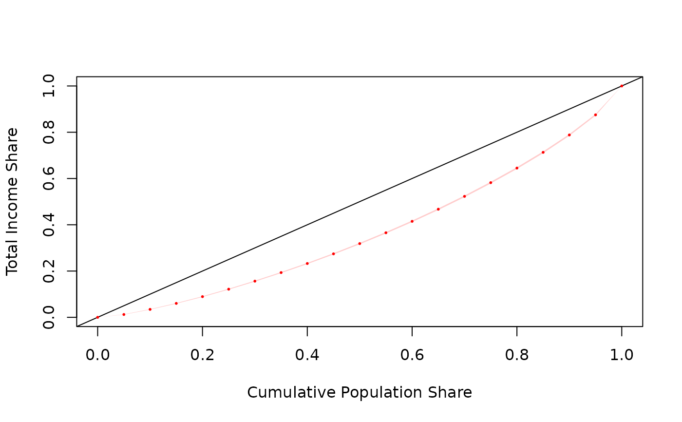 #> lorenz SE
#> L(0) 0.000000 0.0000
#> L(0.05) 0.012201 0.0003
#> L(0.1) 0.034270 0.0005
#> L(0.15) 0.060176 0.0006
#> L(0.2) 0.089371 0.0007
#> L(0.25) 0.121588 0.0008
#> L(0.3) 0.156320 0.0009
#> L(0.35) 0.193344 0.0010
#> L(0.4) 0.232591 0.0010
#> L(0.45) 0.274359 0.0011
#> L(0.5) 0.318651 0.0012
#> L(0.55) 0.365497 0.0013
#> L(0.6) 0.414892 0.0014
#> L(0.65) 0.467307 0.0014
#> L(0.7) 0.522865 0.0015
#> L(0.75) 0.582081 0.0016
#> L(0.8) 0.645068 0.0016
#> L(0.85) 0.713133 0.0016
#> L(0.9) 0.788237 0.0016
#> L(0.95) 0.875173 0.0014
#> L(1) 1.000000 0.0000
# replicate-weighted design
des_eusilc_rep <- as.svrepdesign( des_eusilc , type = "bootstrap" )
des_eusilc_rep <- convey_prep( des_eusilc_rep )
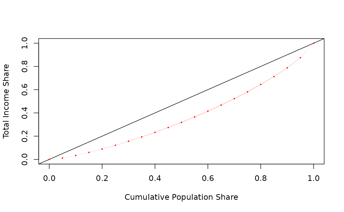
svylorenz( ~eqincome , des_eusilc_rep, seq(0,1,.05), alpha = .01 )
#> lorenz SE
#> L(0) 0.000000 0.0000
#> L(0.05) 0.012201 0.0003
#> L(0.1) 0.034270 0.0005
#> L(0.15) 0.060176 0.0006
#> L(0.2) 0.089371 0.0007
#> L(0.25) 0.121588 0.0008
#> L(0.3) 0.156320 0.0009
#> L(0.35) 0.193344 0.0010
#> L(0.4) 0.232591 0.0010
#> L(0.45) 0.274359 0.0011
#> L(0.5) 0.318651 0.0012
#> L(0.55) 0.365497 0.0013
#> L(0.6) 0.414892 0.0014
#> L(0.65) 0.467307 0.0014
#> L(0.7) 0.522865 0.0015
#> L(0.75) 0.582081 0.0016
#> L(0.8) 0.645068 0.0016
#> L(0.85) 0.713133 0.0016
#> L(0.9) 0.788237 0.0016
#> L(0.95) 0.875173 0.0014
#> L(1) 1.000000 0.0000
# replicate-weighted design
des_eusilc_rep <- as.svrepdesign( des_eusilc , type = "bootstrap" )
des_eusilc_rep <- convey_prep( des_eusilc_rep )
svylorenz( ~eqincome , des_eusilc_rep, seq(0,1,.05), alpha = .01 )
 #> lorenz SE
#> L(0) 0.000000 0.0000
#> L(0.05) 0.012201 0.0003
#> L(0.1) 0.034270 0.0005
#> L(0.15) 0.060176 0.0006
#> L(0.2) 0.089371 0.0008
#> L(0.25) 0.121588 0.0009
#> L(0.3) 0.156320 0.0010
#> L(0.35) 0.193344 0.0012
#> L(0.4) 0.232591 0.0013
#> L(0.45) 0.274359 0.0014
#> L(0.5) 0.318651 0.0015
#> L(0.55) 0.365497 0.0016
#> L(0.6) 0.414892 0.0016
#> L(0.65) 0.467307 0.0017
#> L(0.7) 0.522865 0.0017
#> L(0.75) 0.582081 0.0017
#> L(0.8) 0.645068 0.0016
#> L(0.85) 0.713133 0.0015
#> L(0.9) 0.788237 0.0014
#> L(0.95) 0.875173 0.0011
#> L(1) 1.000000 0.0000
if (FALSE) {
# linearized design using a variable with missings
svylorenz( ~py010n , des_eusilc, seq(0,1,.05), alpha = .01 )
svylorenz( ~py010n , des_eusilc, seq(0,1,.05), alpha = .01, na.rm = TRUE )
# demonstration of `curve.col=` and `add=` parameters
svylorenz( ~eqincome , des_eusilc, seq(0,1,.05), alpha = .05 , add = TRUE , curve.col = 'green' )
# replicate-weighted design using a variable with missings
svylorenz( ~py010n , des_eusilc_rep, seq(0,1,.05), alpha = .01 )
svylorenz( ~py010n , des_eusilc_rep, seq(0,1,.05), alpha = .01, na.rm = TRUE )
# database-backed design
library(RSQLite)
library(DBI)
dbfile <- tempfile()
conn <- dbConnect( RSQLite::SQLite() , dbfile )
dbWriteTable( conn , 'eusilc' , eusilc )
dbd_eusilc <-
svydesign(
ids = ~rb030 ,
strata = ~db040 ,
weights = ~rb050 ,
data="eusilc",
dbname=dbfile,
dbtype="SQLite"
)
dbd_eusilc <- convey_prep( dbd_eusilc )
svylorenz( ~eqincome , dbd_eusilc, seq(0,1,.05), alpha = .01 )
# highlithing the difference between the quantile-based curve and the empirical version:
svylorenz( ~eqincome , dbd_eusilc, seq(0,1,.5), empirical = TRUE, ci = FALSE, curve.col = "green" )
svylorenz( ~eqincome , dbd_eusilc, seq(0,1,.5), alpha = .01, add = TRUE )
legend( "topleft", c("Quantile-based", "Empirical"), lwd = c(1,1), col = c("red", "green"))
# as the number of quantiles increases, the difference between the curves gets smaller
svylorenz( ~eqincome , dbd_eusilc, seq(0,1,.01), empirical = TRUE, ci = FALSE, curve.col = "green" )
svylorenz( ~eqincome , dbd_eusilc, seq(0,1,.01), alpha = .01, add = TRUE )
legend( "topleft", c("Quantile-based", "Empirical"), lwd = c(1,1), col = c("red", "green"))
dbRemoveTable( conn , 'eusilc' )
dbDisconnect( conn , shutdown = TRUE )
}
#> lorenz SE
#> L(0) 0.000000 0.0000
#> L(0.05) 0.012201 0.0003
#> L(0.1) 0.034270 0.0005
#> L(0.15) 0.060176 0.0006
#> L(0.2) 0.089371 0.0008
#> L(0.25) 0.121588 0.0009
#> L(0.3) 0.156320 0.0010
#> L(0.35) 0.193344 0.0012
#> L(0.4) 0.232591 0.0013
#> L(0.45) 0.274359 0.0014
#> L(0.5) 0.318651 0.0015
#> L(0.55) 0.365497 0.0016
#> L(0.6) 0.414892 0.0016
#> L(0.65) 0.467307 0.0017
#> L(0.7) 0.522865 0.0017
#> L(0.75) 0.582081 0.0017
#> L(0.8) 0.645068 0.0016
#> L(0.85) 0.713133 0.0015
#> L(0.9) 0.788237 0.0014
#> L(0.95) 0.875173 0.0011
#> L(1) 1.000000 0.0000
if (FALSE) {
# linearized design using a variable with missings
svylorenz( ~py010n , des_eusilc, seq(0,1,.05), alpha = .01 )
svylorenz( ~py010n , des_eusilc, seq(0,1,.05), alpha = .01, na.rm = TRUE )
# demonstration of `curve.col=` and `add=` parameters
svylorenz( ~eqincome , des_eusilc, seq(0,1,.05), alpha = .05 , add = TRUE , curve.col = 'green' )
# replicate-weighted design using a variable with missings
svylorenz( ~py010n , des_eusilc_rep, seq(0,1,.05), alpha = .01 )
svylorenz( ~py010n , des_eusilc_rep, seq(0,1,.05), alpha = .01, na.rm = TRUE )
# database-backed design
library(RSQLite)
library(DBI)
dbfile <- tempfile()
conn <- dbConnect( RSQLite::SQLite() , dbfile )
dbWriteTable( conn , 'eusilc' , eusilc )
dbd_eusilc <-
svydesign(
ids = ~rb030 ,
strata = ~db040 ,
weights = ~rb050 ,
data="eusilc",
dbname=dbfile,
dbtype="SQLite"
)
dbd_eusilc <- convey_prep( dbd_eusilc )
svylorenz( ~eqincome , dbd_eusilc, seq(0,1,.05), alpha = .01 )
# highlithing the difference between the quantile-based curve and the empirical version:
svylorenz( ~eqincome , dbd_eusilc, seq(0,1,.5), empirical = TRUE, ci = FALSE, curve.col = "green" )
svylorenz( ~eqincome , dbd_eusilc, seq(0,1,.5), alpha = .01, add = TRUE )
legend( "topleft", c("Quantile-based", "Empirical"), lwd = c(1,1), col = c("red", "green"))
# as the number of quantiles increases, the difference between the curves gets smaller
svylorenz( ~eqincome , dbd_eusilc, seq(0,1,.01), empirical = TRUE, ci = FALSE, curve.col = "green" )
svylorenz( ~eqincome , dbd_eusilc, seq(0,1,.01), alpha = .01, add = TRUE )
legend( "topleft", c("Quantile-based", "Empirical"), lwd = c(1,1), col = c("red", "green"))
dbRemoveTable( conn , 'eusilc' )
dbDisconnect( conn , shutdown = TRUE )
}